Gaussian Process Regression

A Gaussian process model is a probabilistic supervised machine learning model that can be used for regression, classification, among many other things. A Gaussian process regression (GPR) model makes predictions incorporating prior knowledge. Being a Bayesian method, it can provide uncertainty measures of the predictions. E.g., it will predict that tomorrow’s stock price is €100, with a credible interval of e.g. €10.

The Gaussian Process Regression generates a pool of candidate functions (a distribution of functions) that could have generated the observed data, and attempts to find the best match (Bayesian inference). Then it selects the best candidate and proceeds to use that function for predictions on new data

So, let's review the underlying concepts to grasp this nonparametric, Bayesian approach and how it fits a function to represent some sample data points and then uses this function to make predictions on new data.

1. What is a Gaussian Process

A Gaussian Process is a collection of random variables, any finite number of which have a joint Gaussian distribution

So what does the above definition actually mean? Let's break it down. We start by building multivariate joint Gaussian distributions from univariate Gaussians distributions. With the single random variable, \(X_1 \sim N(\mu_1, \sigma_1^2)\), let's append \(X_2 \sim N(\mu_2, \sigma_2^2)\) to get the vector \((X_1, X_2)\). If \(X_1\) and \(X_2\) have covariance \(\sigma_{12}\) this vector will have the joint distribution:

If we continue adding more normally distributed random variables, \(X3,X4,…\) we can easily construct larger multivariate Gaussians, once we have their mean and covariance.

A multivariate Gaussian can then be fully specified by the mean vector and covariance matrix. To generalize this concept of continuously incorporating normally distributed random variables into the same distribution, we need two functions: one function to describe the mean and another to describe the covariance.

This is what the Gaussian Process \(\mathcal{G}\mathcal{P}\) provides: It is specified by a mean function, \(\mu(x)\) and a covariance function \(K(x,x′)\), called the kernel function that returns the covariance between two points and simply measures the similarity between \(x\) and \(x′\). There are many options for the kernel. Some common kernel functions include a constant, linear, square exponential and Matern kernel, as well as a composition of multiple kernels.

Now we are not limited to \(n\) variables for a \(n\)-variate Gaussians, but can model any amount with the \(\mathcal{G}\mathcal{P}\). We write:

In the intro we talked about Gaussian Process Regression being a Bayesian method. How does Bayesian Inference (introduced in the next section) come into play now? Let's think of regression: We want to learn a function that represents some sample data. If we see the data, we could make an appropriate aussumption and try to fit a suitable function; e.g. a linear regression, polynomial regression, etc.

This sort of traditional non-linear regression, however, offers only one function \(f(x)\) which is considered to be the best fit. But what about the other ones that are also pretty good. What if we observed more data, and our fit is not the "best" anymore? Or what if we can't even make any assumptions on how this function should look like? Why not just let the regressor find the most suitable function for us?

That is exactly what a Gaussian Process Regression with Bayesian Inference can do.

Since Gaussian Processes let us describe probability distributions over functions we can use Bayes’ rule to update our distribution of functions by observing some training data

2. What is Bayesian Inference - An Intuitive Example & some Concepts

Statistical inference is the process of drawing conclusions and learnings about the characteristics of a large set of items/individuals called the population by using a representative set of observed data (a random sample). By e.g. deriving estimates (parameters like mean, variance, etc. of the underlying ditribution) and testing hypotheses one tries to infer properties of this population.

Inferential statistics can be contrasted with descriptive statistics. Descriptive statistics is solely concerned with properties of the observed data, and it does not rest on the assumption that the data come from a larger population.

There exist two widely used concepts of statistical inference: namely Frequentist (or so called classical) and Bayesian.

Frequentist inference is a type of statistical inference based on classical theory of probability, where probability is defined as a proportion of the occurence (frequency) of the event in the long run. That's where the name frequentist comes from. Frequentist inference therefore draws conclusions from sample data by means of emphasizing the frequency of findings in the data.

So what's the difference now to Bayesian inference?

The essential difference between Bayesian and Frequentist inference is in how the concept of probability is used differently in both concepts.

Frequentists look at \(P(Data|Parameter)\), where the parameter is fixed, and the sample data is random. Therefore, the frequentist learning is only depended on the given sample data. Frequentist inference therefore draws conclusions from data by means of emphasizing the frequency of findings in the sample data.

Frequentist inference: is the process of determining properties of an underlying distribution via the observation of sample data

The Bayesian looks at \(P(Parameter|Data)\) where the parameter is a random variable, and the data is fixed. Meaning that the parameter is a random variable it follows some specific pattern or distribution. The Bayesian now can incorporate some prior knowledge (subjective probability) called belief in deciding on e.g. the specific distribution or pattern of parameters for better inference. While the Bayesian learning is performed by the prior belief as well as the given data, classical frequentist inference can't incorporate any such concept as the parameter is not a random variable.

So, for a Bayesian, probability is more epistemological. Which means that one's belief of the chance of an event occurring is taken into account. This belief also known as prior probability comes from the previous experience, knowledge, literature, etc.

To sum up: Using Bayesian inference we quantify our beliefs and then later can update it on the basis of available data using Bayes Rule (we will talk about in a bit).

Bayesian inference techniques specify how one should update one’s initial beliefs (represented as probability distributions) upon observing new data.

Bayesian inference might be an intimidating concept but to simplify it is just a method for updating our beliefs about the world based on evidence that we observe. So why did someone have to invent the Bayesian Inference? In one sentence: to update the probability as we gather more data.

2.1 Bayesian Inference - An Intuitive Example

This very intuitive Post runs through a well explained illustrative example of Bayesian Inference and explains the definition from above. As Obama's height has already been guessed in the post, we will focus on Berlusconi's height now. Let's just dive into it:

We are going to adjust our beliefs (in Bayesian terms our posterior belief) about the height of Silvio Berlusconi based on some evidence (in Bayesian terms our prior belief).

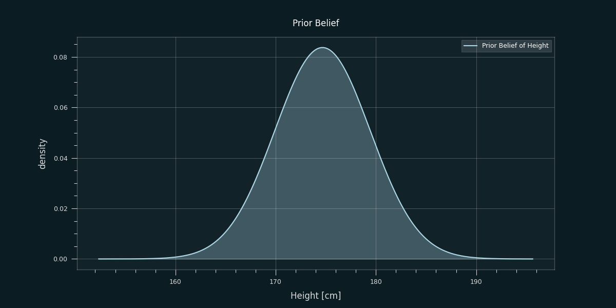
We assume we have never heard of Silvio Berlusconi, or at least we have no idea what his height is. However, we do know that he’s a male white European human being. As stated above we should express our belief about Berlusconi's height (in Bayesian terms we call it prior) before seeing any evidence in form of a probability distribution. So, for simplicity we just choose the the distribution of heights of European males as our initial belief.

Now let’s pretend we can’t just look up Silvio Berlusconi’s height and instead observe some evidence in the form of a picture. Later, the picture will then be our observed data.

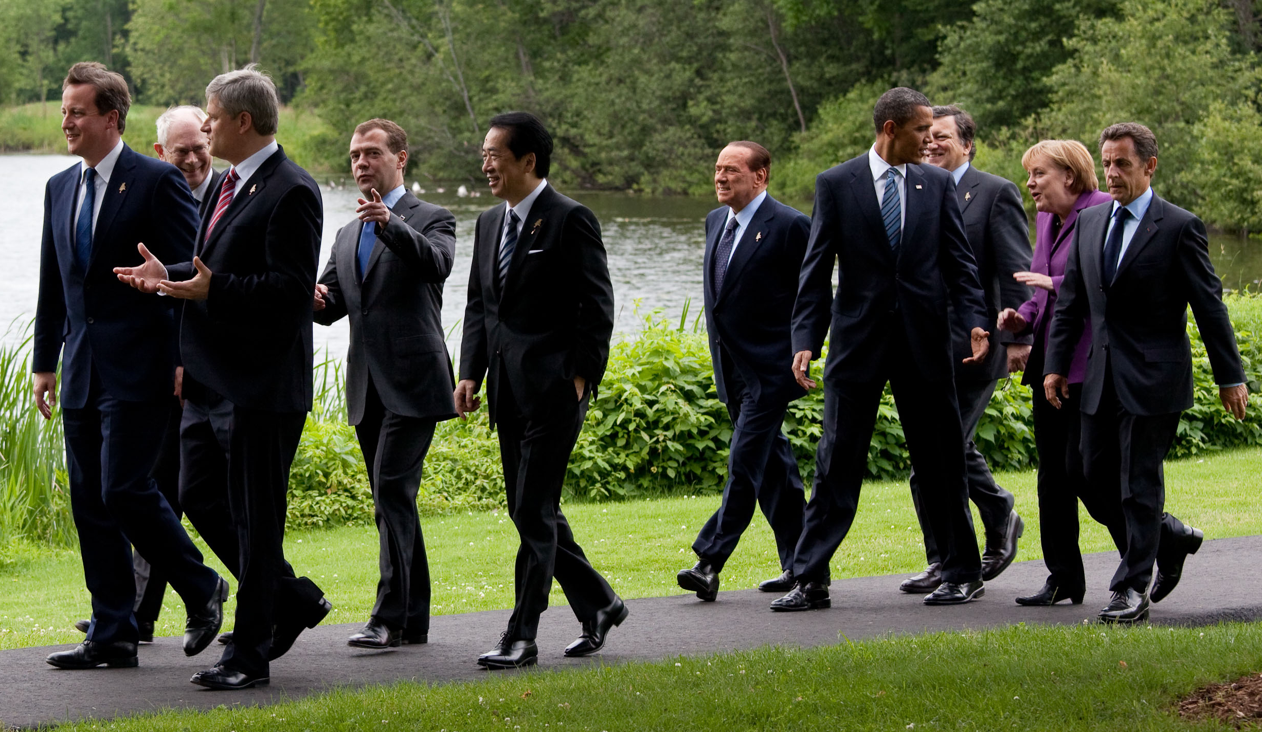
From the above picture we can see that Berlusconi is smaller than average, coming slightly below several other (former) world leaders. However, we can’t be quite sure how tall exactly. The probability distribution shown still reflects/incorporates the chance that he is average height and everyone else in the photo is unusually tall. To become more certain, one could continue looking at more pictures.

Our updated belief in terms of a probability function (in Bayesian terms we call it posterior) looks something like the following now:

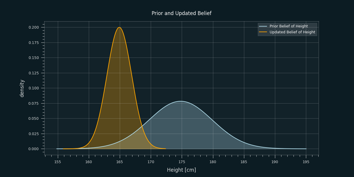
As we can still can not be completely sure that it is only the picture that makes him look smaller due to perspective (or maybe it is even photoshopped) a distribution of belief comes handy to describe the uncertainty that is left estimating Berlusconis height.

2.2 Bayesian Inference - The Formal Concept

As illustrated above, in Bayesian inference our beliefs about the world are typically represented as probability distributions and Bayes’ rule tells us how to update these probability distributions if needed. We may have a prior belief about an event, but our beliefs are likely to change when new evidence in form of data is discovered. That's actually how we use Bayes in everyday life.

Bayes' theorem is used to update the probability (posterior in Bayesian terms) as more evidence or information becomes available (prior in Bayesian terms).

Let's recap Bayes' Theorem in terms of events \(A\) and \(B\):

Where

• \(P(A|B)\) is a conditional probability: the probability of event \(A\) occurring given that \(B\) is true. It is also called the posterior probability of \(A\) given \(B\).
• \(P(B|A)\) is also a conditional probability: the probability of event \(B\) occurring given that \(A\) is true.
• \(P(A)\) and \(P(B)\) are the probabilities of observing \(A\) and \(B\) respectively without any given conditions. They are known as the marginal probabiliy or prior probability.
• \(A\) and \(B\) have to be different events

We can also express Bayes’ Theorem in terms of a probability distribution \(f\) with parameters \(\Theta\) for our modelling purposes:

Where,

• \(\Theta\) are the parameters of the distribution.
• \(\mathcal{D}\) is the observed data.
• \(f(D|\Theta)\) is the likelihood function that models the probability of observing the data for a fixed choice of parameters.
• \(f(\Theta)\) is the prior distribution of the model parameters

Bayes' Theorem states that the posterior is proportional to the likelihood times the prior:

This leads to the following statement describing the purpose of Bayesian Inference:

The core of Bayesian Inference is to combine two different distributions (likelihood and prior) into one “smarter” distribution (posterior)

3. How can we incorporate the concepts from Bayesian Inference to apply a GPR regression

Since Gaussian processes let us describe probability distributions over functions, we can use Bayes’ rule to update our distribution of functions by observing some training data. To reinforce this intuition let's run through an example of Bayesian inference with Gaussian processes that is exactly analogous to the illustrative example from above. Instead of updating our belief about Berlusconis’s height based on a picture, we’ll update our belief about an unknown function given some samples from that function.

With Gaussian Processes we seek to find the most likely function that could produce our data using a Bayesian approach.

Let's recapture the example of regression from above: We want to find the unknown function (line) \(f\) from some data \(D=(x,y)\) that represents this set of data points as closely as possible. Additionally. we want to estimate the uncertainty of our best guess. Let's start applying Bayes' Theorem to do so:

Below we see a visualization of our prior belief about this unknown function as we didn't observe any data yet.

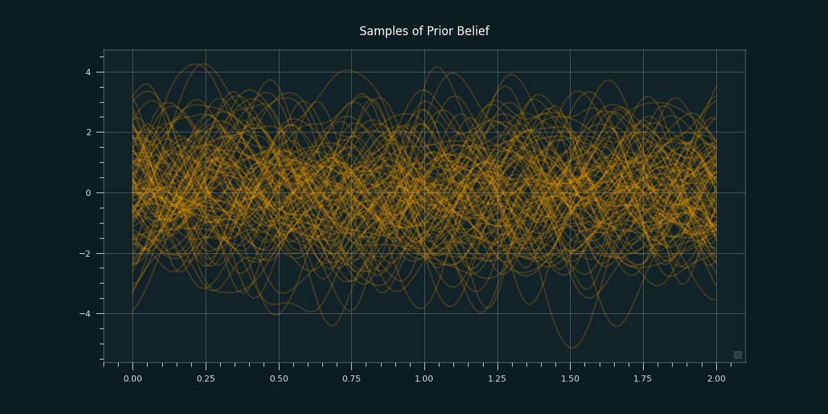
Instead of seeing some picture of Berlusconi, we will observe some outputs of the unknown function at various data points. As stated before, Gaussian processes let us describe probability distributions over functions. Now that we’ve seen some evidence let’s use Bayes’ rule to update our belief about the function to get the posterior Gaussian process aka our updated belief about the function we’re trying to fit.

To get the posterior distribution over functions we need to restrict this joint prior distribution to contain only those functions which agree with our sample data. This literally means we draw random functions from the prior, and reject those that don’t agree with the sample data. In the following we see 10 in the first graph, and 100 samples of our updated belief in the second graph.

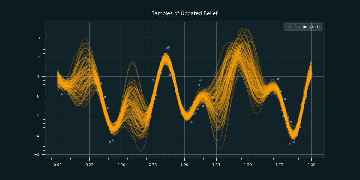
Similarily to the updated and narrowed distribution of possible heights of Silvio Berlusconi we see a narrower distribution of functions as we incorporate the data. The updated Gaussian process is constrained to the possible functions that fit our training data. The lack of knowledge where we don't have any data points is clearly reflected.

Kernels

Recall that in order to set up our distribution, we need to define \(\mu\) and \(K\). In Gaussian processes it is often assumed that \(\mu = 0\), which simplifies the necessary equations.

A great benefit of Gaussian processes is that you can incorporate prior knowledge to model the desired shape of the function via the choice of a Kernel. That means when using a GPR model you can shape your prior belief via the choice of kernel. A full explanation of is beyond the scope of this post.

Advantages and disadvantages of GPs

GPs provide a machine learning approach where uncertainty in the model is concretely available and the model can be used to gain physical insight into the process. Quantifying uncertainty makes them a highly valuable tool compared to most other ML methods. One typical argument against the Bayesian is that the prior can be arbitrary. You pick a prior, I pick a prior. If everyone picks a different prior then we will all get different results (even worse, one could intentionally choose a prior that gives one an answer one wants regardless of the data). Additionally, Bayesian Inference is a computationally quite intensive method.

Let's fit a GPR to our data

We are using GPyTorch to apply a Gaussian Process Regression to our sample data.

import math
import torch
import gpytorch
import numpy as np
from matplotlib import pyplot as plt
import seaborn as sns
from qbstyles import mpl_style

# Plot styling
sns.set_style(
    rc={'axes.facecolor': '.9', 'grid.color': '.8'}
)
sns.set_palette(palette='deep')
%matplotlib inline
plt.rcParams['figure.figsize'] = [12, 6]
plt.rcParams['figure.dpi'] = 100

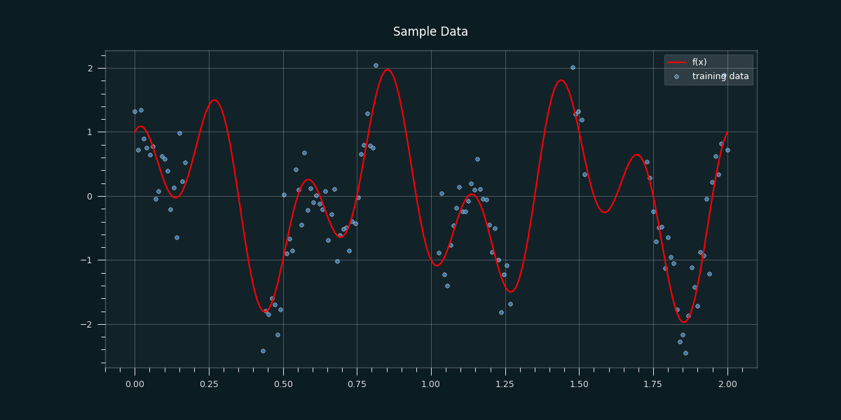
Let's start creating some sample data we want to train or model with. We will create a function we want our data to rely on with some error. Additionally, we create missing values in the data to explore how our GPR model deals with uncertainty.

# Dimension & number of Samples
d = 1
n = 200
# Number of samples (training data)
x = np.linspace(start=0, stop=2, num=n)

# Function to create training data to follow a specific function
def f(x):
    f = np.sin((3*np.pi)*x) + np.cos((7*np.pi)*x)
    return(f)

# True function our samples should be based on
f_x = f(x)

# NaN-statistics definition to create some gaps in the data x
nan_ratio = 0.5
nan_seq_len = 20
number_of_nan_seq = int(nan_ratio * x.size / nan_seq_len)
nan_position = np.random.randint(0, x.size-nan_seq_len, size=number_of_nan_seq)

# Insert NaNs according to NaN-statistics
nan_indexes = np.ones([nan_position.size, nan_seq_len]) * nan_position[:, np.newaxis] + np.arange(0, nan_seq_len)
x_shape = x.shape
x_flat = x.flatten()
x_flat[nan_indexes.astype('int')] = np.nan
x = x_flat.reshape(x_shape)

# Error standard deviation. 
sigma_n = 0.4
# Errors.
epsilon = np.random.normal(loc=0, scale=sigma_n, size=n)

# Observed target variable with a gaussian error
y = f_x + epsilon

# Sample data with missing values deleted
y = y[~np.isnan(x)]
x = x[~np.isnan(x)]

# Final sample data ready for the model
x_train = torch.tensor(x.astype(np.float32))
y_train = torch.tensor(y.astype(np.float32))

Let's plot our sample data:

# Initialize plot
mpl_style(dark=True)
fig, ax = plt.subplots()
# Plot training data.
sns.scatterplot(x=x, y=y, color='#3776ab',label='training data', ax=ax);
# Plot "true" function
sns.lineplot(x=np.linspace(start=0, stop=2, num=n), y=f_x, color='red', label='f(x)', ax=ax);

ax.set(title='Sample Data')
ax.legend(loc='upper right');

Now let's define our model with a RBF-Kernel:

# We will use the simplest form of GP model, exact inference
class ExactGPModel(gpytorch.models.ExactGP):
    def __init__(self, x_train, y_train, likelihood):
        super(ExactGPModel, self).__init__(x_train, y_train, likelihood)
        self.mean_module = gpytorch.means.ConstantMean()
        self.covar_module = gpytorch.kernels.ScaleKernel(gpytorch.kernels.RBFKernel())

    def forward(self, x):
        mean_x = self.mean_module(x)
        covar_x = self.covar_module(x)
        return gpytorch.distributions.MultivariateNormal(mean_x, covar_x)

# Initialize likelihood and model
likelihood = gpytorch.likelihoods.GaussianLikelihood()
model = ExactGPModel(x_train, y_train, likelihood)

# Put the model into training mode
model.train()
likelihood.train()

Let's train the model with 100 iterations

# Use the adam optimizer
optimizer = torch.optim.Adam(model.parameters(), lr=0.1)  # Includes GaussianLikelihood parameters

# "Loss" for GPs - the marginal log likelihood
mll = gpytorch.mlls.ExactMarginalLogLikelihood(likelihood, model)

# Set the number of training iterations
n_iter = 100
for i in range(n_iter):
    # Zero gradients from previous iteration
    optimizer.zero_grad()
    # Output from model
    output = model(x_train)
    # Calc loss and backprop gradients
    loss = -mll(output, y_train)
    loss.backward()
    print('Iter %d/%d - Loss: %.3f   lengthscale: %.3f   noise: %.3f' % (
        i + 1, n_iter, loss.item(),
        model.covar_module.base_kernel.lengthscale.item(),
        model.likelihood.noise.item()
    ))
    optimizer.step()

Let's make some predictions

# Get into evaluation (predictive posterior) mode
model.eval()
likelihood.eval()

# Test data are regularly spaced along [0,2]
# Make predictions by feeding model through likelihood
with torch.no_grad(), gpytorch.settings.fast_pred_var():
    x_test = torch.linspace(0, 2, 1000)
    observed_pred = likelihood(model(x_test))

Let's plot our predictions

with torch.no_grad():

    # Initialize plot
    mpl_style(dark=True)
    fig, ax = plt.subplots()
    # Get upper and lower confidence bounds
    lower, upper = observed_pred.confidence_region()
    # Plot training data as black stars
    sns.scatterplot(np.squeeze(x_train), np.squeeze(y_train), color='#3776ab', label='training data')
    # Plot predictive means as blue line
    sns.lineplot(np.squeeze(x_test), observed_pred.mean.numpy(),color='orange', label='prediction', linewidth = 2)
    # Shade between the lower and upper confidence bounds
    ax.fill_between(x_test.numpy(), lower.numpy(), upper.numpy(), alpha=0.3, color = 'orange', label='Credible Interval')
    ax.legend(['Mean','Observed Data','Credible Interval'], loc='upper right')

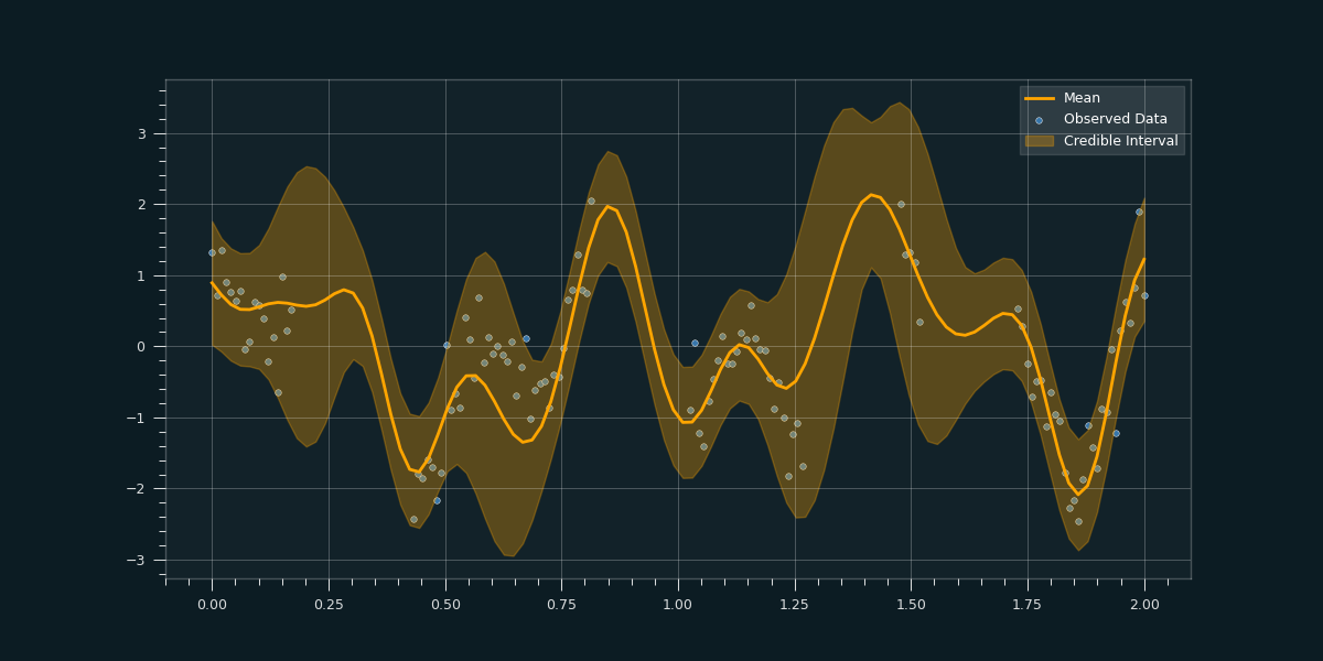
One can clearly see, how the model takes the uncertainty into account where less sample data exists.

Resources

For a more detailed explanations check out the nice post Gaussian Processes, not quite for dummies or this lovely visual exploration of gaussian processes. A step by step coding tutorial or this introductional post and the publication An Intuitive Tutorial to Gaussian Processes Regression by Jie Wang, 2021 might also be very helpful.